“Learning is not attained by chance, it must be sought for with ardor and attended to with diligence.” - Abigail Adams
Trial and error is a fundamental part of living. Every action has consequences that affects us and our surroundings. Learning from our action is important for humans as a way of growing. This is also a key concept in Reinforcement Learning. Trough reinforcement learning, a machine can learn to perform meticolous action based on its “memory”. What could seems like the advent of Skynet is nothing more than basic concepts of algebra, calculus and a lot of probability . With this post I’m going to shed some light over the basics of reinforcement learning, focusing on the difference between on-policy and off-policy algorithms. I will also make use of some code in python to show a simple implementation of reinforcement learning, so feel free to play a bit with the code! You can find everything you need in this Github repository.
Reinforcement Learning: basic concepts
Instead of learning from approximating a function/structure of the labels, in reinforcement learning the model (also called agent) make an action in the environment and see the consequences. Learning is based on the assumption of operant conditioning: specific consequences are associated with voluntary behaviour. In particular, rewards are introduced as a way to increase certain behaviours, while punishment are introduced to decrease other behaviours. This can be formalized in the so-called
Markov Decision Process
A Markov decision process is defined as a 4-tuple $(S, A,P_a ,R_a )$ , where:
- $S$ is a finite set of states;
- $A$ is a finite set of actions;
- $P_a$ is the probability that the agent will move from the state $s$ to the state $s^{\prime}$ after performing the action $a$;
- $R_a$ is the immediate reward (or expected immediate reward) received from moving from $s$ to $s^{\prime}$ after performing the action $a$.
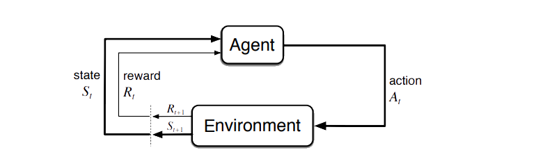
The agent is trying to maximise the reward by taking the correct action. In particular, maximizing the instantaneous reward is not always the correct action. To learn more complex behaviour, the agent needs to learn over time. Thus, the agent tries to maximize the long-term expected reward, which is defined as
where $\gamma$ is a parameter called discount between $0 \leq \gamma < 1$ used to represents the foresightedness of the agent. The presence of delayed rewards makes however the task more complex: it is hard to link the reward with the past actions that led to it. We can define the value function of a state as the expected reward in the state as
We can now unpack the long-term reward to get the Bellman equation:
Both these equations require full knowledge of the policy $\Pi$ of the agent. The policy is a function that maps actions into states:
And to find the optimal policy is the objective of the learner. The Bellman equation then becomes:
So the optimal solution to a Markov decision problem is dynamic programming: you take the bellman equation directly and you solve it for the policy. This however has 2 shortcomings:
- The complexity is exponential;
- The values of $p(s^{\prime} \vert s, a)$ and $R(s,a)$ needs to be known in advance.
What we do then is temporal difference learning: starting from a default estimate of the value function for each state-action pair, which we call Q-value, and improve it over time by making decisions and seeing what happens. This approach is model free (we just need the definition of the state and the knowledge of which state we’re in). In particular, we use the Q-value of the next state as an estimate of future value (bootstrap). Therefore we define the new estimate as
where $Q(s_t,a_t)$ is the old value, $\alpha$ is the learning rate, $r_t$ is the reward, $\gamma$ is the discount factor and $max_{a}Q(s_{t+1},a )$ is the estimate of the optimal future value. In particular, the sum
express the learned value. This formula is guaranteed to converge if $\alpha$ respects some basic properties (the sum diverges, but the sum of squares converges). This is a good time to introduce the concept of
Policies
In the previous formula, we took the action $a$ which maximizes the instantaneous reward at each step. This is a greedy update policy. Other than the update policy, we also have the so-called behavior policy, which is the criteria used to select the next action each state. The most common behaviour policies are:
- $\varepsilon$-greedy: select the $a$ with highest reward with probability $\varepsilon$, or a non-greedy action with probability $1-\varepsilon$;
- softmax: select $a$ based on the softmax distribution of the Q-values.
In both cases, there is some randomness to explore the state and action spaces. For example, the parameter $\varepsilon$ in $\varepsilon$-greedy express the trade-off between exploration and exploitation. $\varepsilon$ should start higher (thus prefer exploring) then gradually decrease (exploit knowledge of the environment which lead to better rewards). In the softmax policy, there is a vector of Q-values for each action, and the learner select the action based on the temperature. High temperature will equal to a uniform distribution, while zero temperature is the greedy action. We’ll need to change the temperature over time to ensure a good learning. The advantage of softmax over $\varepsilon$-greedy is that the learner makes smarter decision when it explore. In particular, we say that an agent is
- On-policy if the update policy and the behaviour policy coincide;
- Off-policy if the update policy and the behaviour policy are different;
The off-policy algorithms have an advantage, since they can take more risks, as they assume they won’t make mistakes in the next step. The best algorithm for reinforcement learning at the moment are:
- Q-learning: off-policy algorithm which uses a stochastic behaviour policy to improve exploration and a greedy update policy;
- State-Action-Reward-State-Action (SARSA): on-policy algorithm which uses the stochastic behaviour policy to update its estimates.
The formula to estimate the new value for an on-policy algorithm like SARSA is
which is similar to what we’ve already seen, except we are not updating anymore the action trough greedy policy.
Q-learning and SARSA implementation
The best way to grasp the difference between the two algorithms is to put what I’ve just explained into practice. To do this, we create a simple Markovian environment where our agent needs to reach a goal, which is a fixed state in the environment. Surpassing the boundaries (going outside the $10\times 10$ map) lead to a negative reward. Since this is quite the easy task for our learner, we also add a “pit”, which involves a penalty when crossed. You can find the code for the environment here. Since it’s nothing special, I will leave the exploration of the class on you. We are more interested in how to implement different algorithms and policies. Let’s examine the code for programming our agent. The first to do is initializing the agent:
1
2
3
4
5
6
7
8
9
10
11
12
13
14
15
# agent which can move over the environment
class Agent:

    # initialize
    def __init__(self, states, actions, discount, max_reward, softmax, sarsa):
        self.states = states
        self.actions = actions
        self.discount = discount
        self.max_reward = max_reward
        self.softmax = softmax
        self.sarsa = sarsa
        # initialize Q table
        # Q-table is a actions/states matrix used to select which action perform;
        # The value of each cell will be the maximum expected future reward for that given state and action.
        self.qtable = np.ones([states, actions], dtype=float) * max_reward / (1 - discount)
The part we’re interested the most in is the Q-table initialization: here we’ll calculate the maximum expected future reward for each action at each state, also called Q-values. Those values are then improved over time as our agent performs action in the environment. The behaviour policy is updated trough this function:
1
2
3
4
5
6
7
8
9
10
11
12
13
# action policy: implements epsilon greedy and softmax
    def select_action(self, state, epsilon):
        qval = self.qtable[state]
        prob = []
        if self.softmax:
            # use Softmax distribution
            prob = sp.softmax(qval / epsilon)
        else:
            # assign equal value to all actions
            prob = np.ones(self.actions) * epsilon / (self.actions - 1)
            # the best action is taken with probability 1 - epsilon
            prob[np.argmax(qval)] = 1 - epsilon
        return np.random.choice(range(0, self.actions), p=prob)
We can implement the softmax distribution using scipy.special.softmax, where “qval” is the Q-value of the state our agent is currently in, and “epsilon” is the $\varepsilon$ parameters discussed before. To implement the $\varepsilon$-greedy policy instead, we assign equal probability to all the actions our agent can take from the current state, while the action with maximum reward is taken with probability $1-\varepsilon$. If we want to use the greedy policy, we just set epsilon to zero. This way, we’ll always take the maximum reward action. The following function is sued to update the Q-values after each action:
1
2
3
4
5
6
7
8
9
10
11
12
 # update function (Sarsa and Q-learning). This occurs every time an episode is done.
    def update(self, state, action, reward, next_state, alpha, epsilon):

        # find the next action (greedy for Q-learning, using the decision policy for Sarsa)
        if self.sarsa:
            next_action = self.select_action(next_state, epsilon)
        else:
            next_action = self.select_action(next_state, 0)
        # calculate long-term reward with bootstrap method
        observed = reward + self.discount * self.qtable[next_state, next_action]
        # bootstrap update
        self.qtable[state, action] = self.qtable[state, action] * (1 - alpha) + observed * alpha
The bootrap method used to update the Q-values is the same formula we’ve already saw during my introduction on reinforcement learning concepts above. The training of the agent is based on the Q-table I’ve mentioned previously. Every episode, the agent is “free” to move for a fixed numbers of actions (the episode length). The action is selected by the agent depending on the algorithm and the policy in use. Then, the long-term reward gets calculated using bootstrap methods, and the Q-table gets updated. The code will look something like this:
1
2
3
4
5
6
7
8
9
10
11
12
13
14
15
16
17
18
19
20
21
22
23
24
25
26
27
28
29
30
# perform the training
    for index in range(0, episodes):

        initial = [np.random.randint(0, x), np.random.randint(0, y)]

        # initialize environment
        state = initial
        env = environment.Environment(x, y, state, goal, pit, labyrinth)
        reward = 0

        # run episode
        for step in range(0, episode_length):
            # find state index
            state_index = state[0] * y + state[1]

            # choose an action
            action = learner.select_action(state_index, epsilon[index])

            # the agent moves in the environment
            result = env.move(action)

            # Q-learning update
            next_index = result[0][0] * y + result[0][1]
            learner.update(state_index, action, result[1], next_index, alpha[index], epsilon[index])

            # update state and reward
            reward += result[1]
            state = result[0]

        reward /= episode_length
You can expect your agent to behave randomly in the early episodes, trying to learn as much as possible from the environment surrounding it.
But give it some time and you can rest assured it will become an ace in reaching the goal!
Both Q-learning and SARSA will lead our agent to the goal, but there are some difference we have to take into account. As I said previously, SARSA is more conservative than Q-learning: thus it will prefer a “longer” path towards the goal (therefore also getting less reward) but safer (it will try to keep distance from what cause the penalties, like the borders or the pit). You can compare the previous pathing of a trained agent using Q-learning with a trained agent using SARSA ($\varepsilon$-greedy policy):
A common way to compare the performance of different algorithms in reinforcement learning is plotting the cumulative reward (the sum of all rewards received so far) as a function of the number of steps.
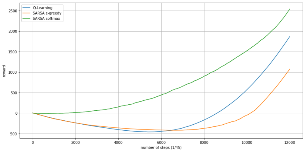
It’s interesting to look at the fact that the rewards are initially going down: this is how much reward must be sacrificed before it starts to improve. In particular, when the zero is crossed the algorithm has recouped its cost of learning. Here it’s clear how sarsa using $\varepsilon$-greedy performs worse than Q-learning in terms of sheer reward. This is because sarsa take a longer route for turning around the pit, resulting in lower reward. More complex policies like Softmax can provide better results, but are not always possible to implement. We can also see that basic algorithm like the greedy Q-learning can still outperform on-policy algorithm like sarsa depending on the situation.
Hope reading this helped you going trough some basic concepts of reinforcement learning. Feel free to fork my repo on Github if you want to try out the code yourself, and leave a star if you find it useful. Stay tuned for more contents!
sources
“Deep Learning”, by Ian Goodfellow and Yoshua Bengio and Aaron Courville
“Reinforcement learning”, by Wikipedia
“Evaluating Reinforcement Learning Algorithms”, by David Poole and Alan Mackworth